Convolution in Continuous Time Signal Using Matlab Code

18-396 SIGNALS AND SYSTEMS
Lab 7: Convolution
Week of March 17-21, 2003

Part 1) The 'conv' command

a) The MATLAB command 'conv' computes the convolution of two vectors. To become familiar with this command, use it to compute some of the convolutions for the discrete-time signals on the "Joy of Convolution" web site www.jhu.edu/~signals/discreteconv2/index.html. To do this, create vectors representing the three discrete-time signals (beginning at n=0, the first non-zero value for each signal), and compute the convolutions using the 'conv' command. Define your signals in an m-file, or save them so that you can reload them so that you can show the TA your work. Plot your results with the correct values of n on the horizontal axis. (Since MATLAB always starts vector indices at 1, you will have to introduce a separate vector for the values of n.)

b) Suppose the signals in part (a) are shifted in time so that the first non-zero value of the signal x starts at nx and the first nonzero value of h is nh, where nx and nh are arbitrary integers. Write an m-file that plots x, h, and conv(x,h) with the correct time indices. To run this m-file, you will first set x and h to one of the three vectors of values from part (a), and assign values to nx and nh. Then running the m-file will make the three plots. Create two new additional signals of your choice for x and h to test and demonstrate your convolution of arbitrarily shifted functions.

c) Now look at the examples of continuous-time convolution at the "Joy of Convolution" web site www.jhu.edu/~signals/convolve/index.html. To use 'conv' for continuous-time signals, the vectors representing the continuous-time signals are the values of the signals sampled at some period T. The convolution integral can then be approximated by thinking of the sum performed by 'conv' as a Riemann sum. Therefore, the sum must be multiplied by T to reflect the width of the sampling interval. Letting T=0.01, create vectors representing the three continuous-time signals on the "Joy of Convolution" web site, starting at t = 0 for each signal. Then, perform the continuous-time convolutions using 'conv' and plot the result. Introduce an appropriate vector of time values so that the horizontal axis of your plot is correct. Note: Compare your results with the convolutions on the web site to make sure you have correctly scaled the convolution sum.

Part 2) Using convolution for filtering
(This problem was found at http://www.swarthmore.edu/NatSci/echeeve1/Class/e71/E71L3/E71L3.html)

A Chirp signal

Create a chirp signal that goes from 0 to 2 kHz in 10 seconds (i.e., the frequency increases at 200 Hz/sec).�(All of these commands are in the file Lab7_matlab_code.m).

FS=8000;
DT=1/FS;
Tfinal=10.0;
t=0:DT:Tfinal;

Finitial=0;
Ffinal=2000;

y=chirp(t,Finitial,Tfinal,Ffinal);
sound(y,FS);

You can visualize the increasing frequency with a spectrogram (note that the maximum frequency on the spectrogram is 4000 Hz because the sampling frequency was 8000 Hz).

specgram(y,128,FS)

A Bandpass filter

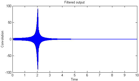
Create a short sinusoidal signal (1/10 second) at 400 Hz, and convolve it with the chirp.���(All of these commands are in the file Lab7_matlab_code.m).�

t1=0:DT:0.1;
f400=sin(2*pi*400*t1).*exp(-40*t1); %A 400 Hz decaying sine wave.

z=conv(y,f400);

%Because z is longer than y, create a new vector
%"n" so we can plot just the beginning part of z.
n=1:length(t);�
plot(t,z(n));
xlabel('Time');
ylabel('Convolution');
title('Filtered output');

The signal (f400) behaves as a bandpass filter -- there is only a significant output around t=2 seconds, when the frequency of the chirp is about 400 Hz.�� Why would you expect the sinusoidal signal to act as a bandpass system?

DTMF Signals

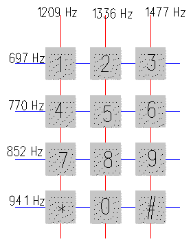
The picture below shows a typical touch-tone phone pad.� When you press a button you generate a tone that is the sum of the column frequency and the row frequency.�� For example, if you hit the key "9", you generate a tone that is the sum of a 1477 Hz sine wave and a 852 Hz sine wave because "9" is at the intersection of that row and column.� This is called the DTMF (Dual-Tone Multiple-Frequency) signalling scheme.

Put the file touchtone.wav in your Matlab working directory.� Load the sequence into your computer and play it.��(All of these commands are in the file Lab7_matlab_code.m).

��������� [ttone,FS,bits]=wavread('touchtone');
��������� soundsc(ttone,FS)

a) Use several bandpass filters to determine the phone number in touchtone.wav.� Make sure you clearly and neatly present your results.� You can use a single plot with several subplots. Prepare a set of plots to explain to the TA how you solved this problem.

b) Verify your results from part (a) by taking a spectrogram of the touchtone signal.� You should experiment with the NFFT variable to get the best result.� (NNFT equals 128 in the example with the chirp signal, above.)

�

---

cupplesbeenarile.blogspot.com

Source: https://users.ece.cmu.edu/~krogh/18396/lab7_convolution.html

Share this post